Introduction to Pure See. © Marius Buliga (2020-2021), https://mbuliga.github.io/quinegraphs/puresee.html
All chemlambda projects
Pure See
is a geometrical, or cartographical lambda calculus. As primitives it uses variables, terms and a small number of special words: from, see, as, in, apply, with, note, over, free, origin.Contents
Scalars
Variables and terms
Commands
Conversion between commands, functional and algebraic forms
Reduction of trigrams
Multiplication by scalars. Origin
Reduction by passing to the limit
Emergent rewrites
Scalars
(back to contents)
| special word | as a rational function |
|---|---|
| see | see[z] = z |
| from | from[z] = 1-z |
| apply | apply[z] = 1/z |
| with | with[z] = 1/(1-z) |
| note | note[z] = z/(z-1) |
| over | over[z] = (z-1)/z |
| as | as[z] = -1 |
| in | in[z] = 1 |
These scalars (with the exception of those special ones) generate all the scalars via two operations: composition of scalars and multiplication of scalars.
Composition of scalars is defined as composition of functions
k[l][z] = k[l[z]], for k,l scalars
Multiplication of scalars is defined as multiplication of functions
[k l][z] = k[z] l[z], for k,l scalars
Variables and terms
(back to contents)
Variables are denoted by a, b, c, ... A term is either a variable or the result of an operation between terms. There are 6 operations: ◦ is "map" , • is "unmap", (lambda calculus style) abstraction, (lambda calculus style) application, > is "fi", < is "fox". All in all, a term is defined as:| origin | | | (is asimilated with a variable) | ||
| a | variable | | | ||
| a ◦ b | a, b terms | | | (map) | |
| a • b | a, b terms | | | (unmap) | |
| a > b | a, b terms | | | (fi) | |
| a < b | a, b terms | | | (fox) | |
| λ a. b | a, b terms | | | (abstraction) | |
| a b | b, b terms | | | (application) |
Commands
(back to contents)
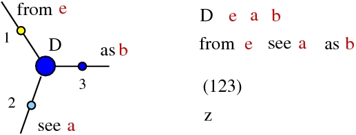
As indicated in the images, each command can be associated to a directed interaction combinators (dirIC) node, as defined in:
[Alife properties of directed interaction combinators vs. chemlambda. Marius Buliga (2020), https://mbuliga.github.io/quinegraphs/ic-vs-chem.html#icvschem]
or a chemlambda [arXiv:2003.14332] node.
For the list of chemlambda rewrites and the history of versions see
[Graph rewrites, from emergent algebras to chemlambda. Marius Buliga (2020), https://mbuliga.github.io/quinegraphs/history-of-chemlambda.html]
The exceptions are the nodes named "D" and "FOX", first time used in kali24 (but see them described in the file chemistry.js) and the node "FIN", the fanin dual to the fanout FO.
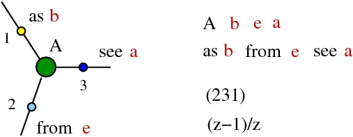
| command | algebraic form | functional form | graphical form |
|---|---|---|---|
|
from e see a as b; |
map
b = e ◦ a; |
from e see a as b; |
|
|
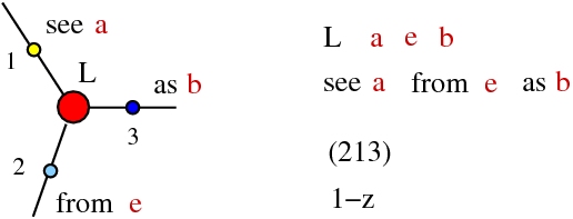
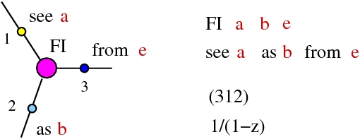
see a from e as b; |
abstraction
b = λ e. a; |
see a from e as b; |
|
|
as b from e see a; |
application
a = b e; |
apply b over e as a; |
|
|
see a as b from e; |
fi
e = a > b; |
note a with b as e; |
|
|
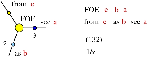
from e as b see a; |
unmap
a = e • b; |
over e apply b as a; |
|
|
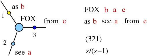
as b see a from e; |
fox
e = b < a; |
with b note a as e; |
|
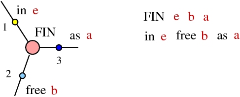
in e as a free b;
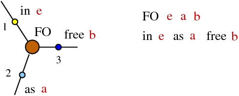
in e free b as a;
in a as b;
in a;
as a;
free a;
Conversion between commands, functional and algebraic forms
(back to contents)
apply b over e as a;
(apply as) (as b from e see a);
| b = a; | is replaced by | in a as b; |
| command | algebraic form | replace by |
|---|---|---|
| from e see a as b; | b = e ◦ a; | in (e ◦ a) as b; |
| see a from e as b; | b = λ e. a; | in (λ e. a) as b; |
| as b from e see a; | a = b e; | in (b e) as a; |
| see a as b from e; | e = a > b; | in (a > b) as e; |
| from e as b see a; | a = e • b; | in (e • b) as a; |
| as b see a from e; | e = b < a; | in (b < a) as e; |
| LHS pattern | action |
|---|---|
| in a as b; | delete the command, replace b by a |
(ALG) and (COMB) may be combined into an evaluation rewrite (EVAL), for example
| LHS pattern | action |
|---|---|
| see a from e as b; | delete the command, replace b by λ e. a |
Reduction of trigrams
(back to contents)
A trigram is any triple of commands of the form:| for[ε] a see[ε] b as[ε] e; |
| for[μ] e see[μ] c as[μ] d; |
| for[ε] u see[ε] w as[ε] c; |
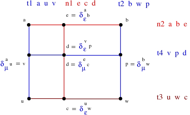
The main rewrite (schema) of Pure See is (SHUFFLE), which replaces a trigram by another trigram:
| LHS pattern | RHS pattern | ||||||||||
|---|---|---|---|---|---|---|---|---|---|---|---|
|
|
Multiplication by scalars. Origin
(back to contents)
from[μ] origin see[μ] T as (μ T);
from[ε] u see[ε] w as[ε] c;
from[ε] (μ u) see[ε] (μ w) as[ε] (μ c);
| LHS pattern | RHS pattern | ||||||||||
|---|---|---|---|---|---|---|---|---|---|---|---|
|
|
Reduction by passing to the limit
(back to contents)
We are allowed to "pass to the limit" with scalars, to one of the special scalars 0, 1, ∞. This passage to the limit is a rewrite.| LHS pattern | RHS pattern | |
|---|---|---|
| from[μ] e see[μ] a as[μ] b; | μ → 1 | in e; in a as b; |
| μ → 0 | in a; in e as b; | |
| μ → ∞ | in e free a as b; | |
| see[μ] a from[μ] e as[μ] b; | μ → 1 | as e; in a as b; |
| μ → 0 | in a as e free b; | |
| μ → ∞ | as b; in a as e; | |
| as[μ] b from[μ] e see[μ] a; | μ → 1 | in e; in b as a; |
| μ → 0 | in b free e as a; | |
| μ → ∞ | as b; in e as a; | |
| see[μ] a as[μ] b from[μ] e; | μ → 1 | in a free b as e; |
| μ → 0 | in a; in b as e; | |
| μ → ∞ | in b; in a as e; | |
| from[μ] e as[μ] b see[μ] a; | μ → 1 | in e as b free a; |
| μ → 0 | as a; in e as b; | |
| μ → ∞ | as b; in e as a; | |
| as[μ] b see[μ] a from[μ] e; | μ → 1 | as e; in b as a; |
| μ → 0 | as a; in b as e; | |
| μ → ∞ | in b; as a free e; |
Emergent rewrites
(back to contents)
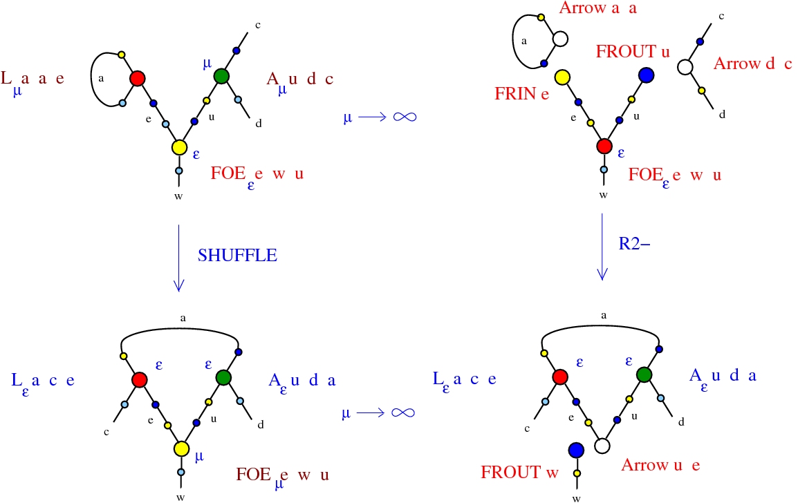
Here is exemplified the rewrite L-A (or the beta rewrite) as an emergent rewrite. You see the rewrite described in graphical form and in trigram form: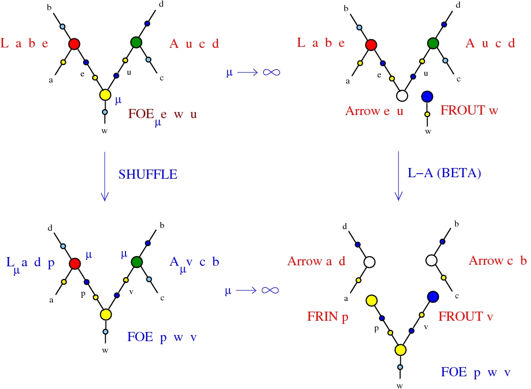
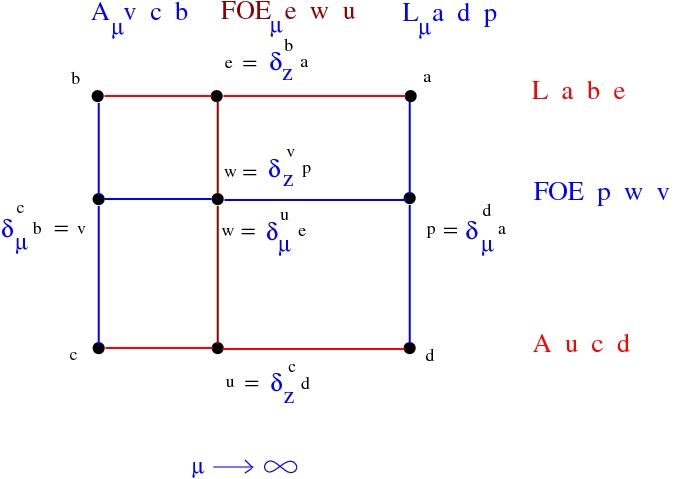
Look in diagonal, from the top left to the bottom right of the figure which shows the graphical form of L-A as emergent. We may interpret the FOE node as the rewrite enzyme.
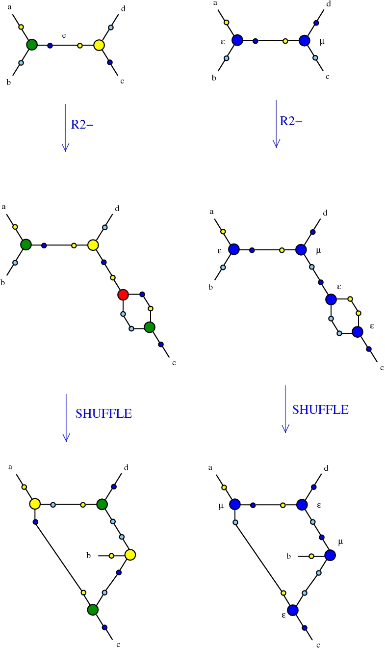
DIST rewrites of chemlambda, dirIC or even those of kali24 are described in the file chemistry.js. They are particular forms of the possible DIST rewrites which are compatible with the SHUFFLE. Here is a tool which generates all possible such rewrites.
Let's concentrate on the dist1 rewrite. The following figure shows the graphical form of this rewrite:
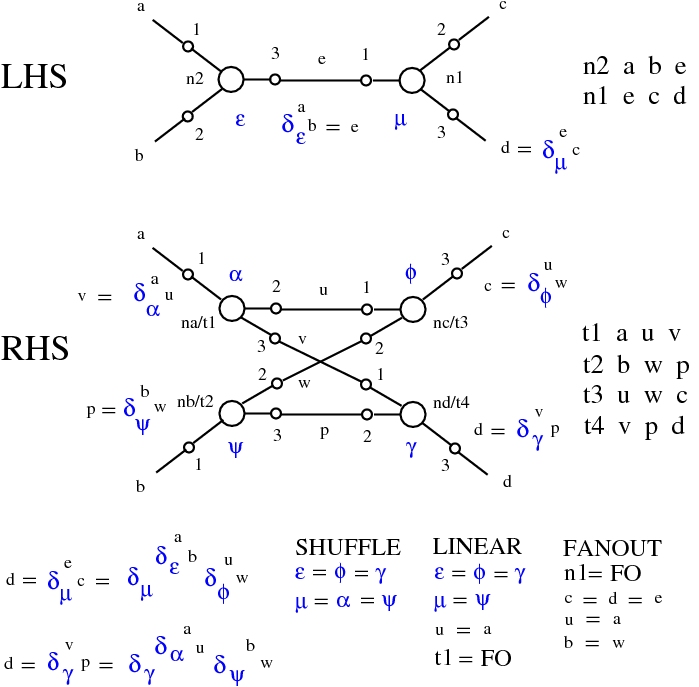
The creation of this new line can be achieved by an emergent Reidemeister 2 rewrite: